Lab 1A - Data, Code & RStudio

Directions: Follow along with the slides, completing the questions in blue on your computer, and answering the questions in red in your journal.

Welcome to the labs!

Throughout the year, you'll be putting your data science skills to work by completing the labs.
You'll learn how to program in the R programming language.

– The programming language used by actual data scientists.
Your code will be written in RStudio which is an easy to use interface for coding using R.

So let's get started!

The data for our first few labs comes from the Centers for Disease Control (CDC).

– The CDC is a federal institution that studies public health.
Type these two commands into your console:
```
data(cdc)
View(cdc)
```
Describe the data that appeared after running View(cdc):

– (1) Who is the information about?

– (2) What sorts of information about them was collected?
To find out more information about the cdc data, type the command below into your console.

– To get back to the slides find and click on the Viewer tab.
```
?cdc
```

Data: Variables & Observations

Data can be broken up into two parts.

`1. Observations

`2. Variables

– Observations are the who or what we are collecting data from/about.

– Variables are the measurements or characteristics about our observations.
If need be, re-type the command you used to View your data. Then answer the following:

– (3) Based on the data, describe a few characteristics about the first observation.

– (4) What does the first column tell us about our observations?
In order to describe the first observation, notice that you had to look at the first row of the spreadsheet. Each row, in this case, describes a person.
The columns of the spreadsheet represent variables.

Uncovering our Data's Structure

Now that we've looked at our data, let's look at how RStudio is organized.
RStudio's main window is composed of four panes
Find the pane that has a tab titled Environment and click on the tab.

– This pane contains a list of everything that's currently available for R to use.

– Notice that R knows we have our cdc data loaded.
(5) How many students are in our cdc dataset?
(6) How many variables were measured for each student?

Some New Functions

Type the following commands into the console:
```
dim(cdc)
nrow(cdc)
ncol(cdc)
names(cdc)
```
(7) Which of these functions tell us the number of observations in our data?
(8) Which of these functions tell us the number of variables?

First Steps

Typing commands into the console is your first step into the larger world of programming or coding (terms which are often used interchangeably).
Coding is all about learning how to send instructions to your computer.

– The way we speak to the computer, using a coding language, is syntax.
R is one of many coding languages. Each coding language is slightly different, and these differences are reflected in the syntax.
Capitalization, spelling and punctuation are REALLY important.

Syntax matters

Run the following commands.

Names(cdc)
NAMES(cdc)
names(cdc)
names(CDC)

(9) What happens after each command?
(10) Which does R understand?

R's most important syntax

Most of the commands you will be using follow the syntax below.
```
function (y ~ x, data = ____ )
```
To create graphs or plots you need to provide R with the following:

– The name of the R function, often the plot’s name, that tells the computer how to create your graph.
- The variable(s) containing the information we want the function to use.
- The dataset containing the variables.
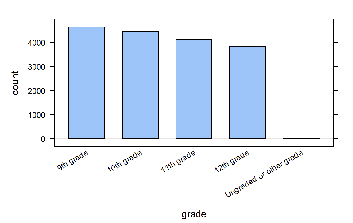
Notice that when we analyze a single variable the value for y is left blank.
```
bargraph(~grade, data = cdc)
```

Later on, we’ll see we can use this syntax to do more than create graphs.

Syntax in action

Search through the different panes. Find and then click on the Plots tab.
- To get back to the slides, find and then click on the Viewer tab.
(11) Would a histogram, bargraph, or scatterplot be useful for answering the question: Is it unusual for students in the CDC dataset to be taller than 1.8 meters?

Run the three commands below then answer the question that follows.

histogram(~height, data = cdc)

bargraph(~height, data = cdc)

xyplot(weight~height, data = cdc)

(12) Do you think it’s unusual for students in the cdc dataset to be taller than 1.8 meters? Why or why not?
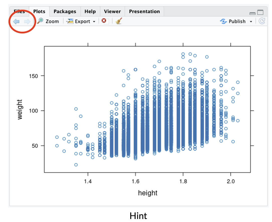
Hint: Use the arrow keys on the Plots tab to toggle between the plots.

On your own:

After completing the lab, answer the following questions:

– (13) What is public health and do we collect data about it?

– (14) How do you think our data was collected? Does it include every high school aged student in the US?

– (15) How might the CDC use this data? Who else could benefit from using this data?

– (16) Write and run the code to visualize the distribution of weights of the students in the CDC data with a histogram. What is the typical weight?

– (17) Write and run the code to create a bargraph to visualize the distribution of how often students ate fruit. About how many students did not eat fruit over the previous 7 days?